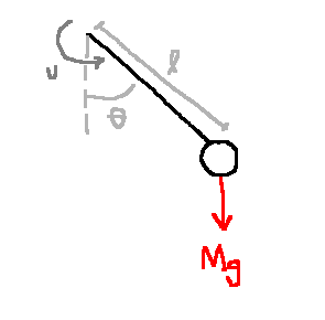
Design a controller to keep the pendulum in upright position.
\[\begin{align} \text{Model:}\\ \dot{x_1}&=x_2\\ \dot{x_2}&= \frac{-g}{l}\sin x_1 + \frac{1}{Ml^2}u\\ y&=x_1\\ \\ \text{Equilibrium config } (\bar{x}, \bar{u}) \text{ at which } y=\pi \text{ is: }\\ (\bar{x}, \bar{u}) &= \left(\begin{bmatrix}\pi\\0\end{bmatrix}, 0\right)\\ \\ \text{Linearization:}\\ \dot{\partial x} &= \begin{bmatrix}0&1\\\frac{g}{l}&0\end{bmatrix} \partial x + \begin{bmatrix}0\\\frac{1}{Ml^2}\end{bmatrix}\partial u\\ \partial x &:= x-\bar{x}\\ \partial u &:= u-\bar{u}\\ \partial y &:= y-\bar{y}\\ &= \begin{bmatrix}1 & 0\end{bmatrix}\partial x\\ \\ \text{Transfer function:}\\ U(s) &:= \mathbb{L}\{\partial u\}, Y(s) := \mathbb{L}\{\partial y\}\\ \\ \text{Poles:}\\ s &= \pm \sqrt{\frac{g}{l}}\\ \\ \frac{Y(s)}{U(s)} = \frac{1}{Ml^2} \frac{1}{s^2 - \frac{g}{l}} =: P(s)\\ \end{align}\]

One controller that does the job is \(C(s) = 100 + \frac{s+10}{s+20}\), a "lead" controller.
With this choice of controller, the TF from \(R\) to \(Y\) is:
\[\frac{Y(s)}{R(s)} = \frac{C(s)P(s)}{1 + C(s)P(s)} = \frac{100s+1000}{s^3 + 20s^2 + 99s + 980}\]
Closed-loop poles: \(\{-17.5, -1 \pm 7.3j\}\)
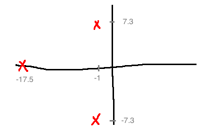
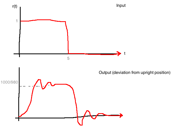
Closed-loop response is dominated by poles at \(s=-1 \pm 7.3j\), making it look like an underdamped second-order system with a lot of overshoot because of the large angle from the x axis.
Input signal: From 0 to 5s, move in the counter-clockwise direction by 1 radian. After 5s, return to the upright position.
To implement the controller, we have the following (A/D means analogue to digital):

In this case, using a "bilinear transformation", we get:
\[u[k] = \frac{1}{2+20T}\left((20T-2)u[k-1]+100(2+10T)e[k]+100(10T-2)e[k-1]\right)\]
Where:

Systems
Signals
What does it mean for this system to be stable?
Assume \(P\) and \(C\) are rational; \(P\) is strictly proper; \(C\) is proper.
Set \(r(t)=d(t)=0\). Bring in state-space models for \(C\) and \(P\).

\[\begin{align} \dot{x_c} &= A_cx_c+B_ce\\ u &= C_cx_c+D_ce\\ \\ \dot{x_p} &= A_p x_p + B_pu\\ y &= C_px_p\\ \end{align}\]
We get:
\[\underbrace{\begin{bmatrix}\dot{x_p}\\\dot{x_c}\end{bmatrix}}_{x_{cl}} = \underbrace{\begin{bmatrix}A_p-B_pD_cC_p&B_pC_c\\-B_cC_p&A_c\end{bmatrix}}_{A_{cl}}\begin{bmatrix}X_p\\x_c\end{bmatrix}\]
The closed-loop system is internally stable if \(\dot{x_{cl}}=A_{cl}x_{cl}\) is asymptotically stable.
Given:
\[\begin{align}
\dot{x_p} &= \begin{bmatrix}0&1\\0&-5\end{bmatrix}x_p + \begin{bmatrix}0\\1\end{bmatrix}u\\
y &= \begin{bmatrix}1&0\end{bmatrix}x_p\\
\dot{x_c} &= -15x_c + e\\
y &= -1000x_c + 100e\\
\end{align}\]
Then:
\[\begin{align}
A_{cl} &= \begin{bmatrix}
\begin{bmatrix}0&1\\0&-5\end{bmatrix}-\begin{bmatrix}0\\1\end{bmatrix}100\begin{bmatrix}1&0\end{bmatrix} &
-\begin{bmatrix}0\\1\end{bmatrix} \\
-\begin{bmatrix}1&0\end{bmatrix} &
-15
\end{bmatrix}\\
&= \begin{bmatrix}0&1&0\\-100&-5&-1000\\-1&0&-15\end{bmatrix}\\
\\
\det(sI-A_{cl}) &= \det\begin{bmatrix}s&-1&0\\100&s+5&1000\\1&0&s+15\end{bmatrix}\\
&= s(s+5)(s+15)+100(s+5)\\
&= (s+5)(s^2+15s+100)\\
\end{align}\]
You can check that all the roots of the determinant (all the eigenvalues) have negative real parts. This implies that \(\dot{x_{cl}}=A_{cl}x_{cl}\) is asymptotically stable, and therefore the feedback system is internally stable.
Given the same feedback loop as before:
This system has 6 transfer functions from \((r, d)\) to \((e, u, y)\). Finding them:
\[\begin{align} Y &= PU\\ E &= R - PU\\ U &= D+CE\\ \Rightarrow \begin{bmatrix}1&P\\-C&1\end{bmatrix}\begin{bmatrix}E\\U\end{bmatrix}&=\begin{bmatrix}R\\D\end{bmatrix}\\ \begin{bmatrix}E\\U\end{bmatrix} &= \frac{1}{1+PC}\begin{bmatrix}1&-P\\C&1\end{bmatrix}\begin{bmatrix}R\\D\end{bmatrix}\\ \\ \frac{E}{R} &= \frac{1}{1+PC}\\ \frac{E}{D} &= \frac{-P}{1+PC}\\ \frac{U}{R} &= \frac{C}{1+PC}\\ \frac{U}{D} &= \frac{1}{1+PC}\\ \frac{Y}{R} &= \frac{PC}{1+PC}\\ \frac{Y}{D} &= \frac{P}{1+PC}\\ \end{align}\]
A feedback system is input-output stable if \((e, u, y)\) are bounded whenever \((r, d)\) are bounded.
Since whenever \(r\) and \(e\) are bounded, so is \(y=r-e\), we only need to look at the TFs from \((r,d)\) to \((e,u)\).
\[P(s)=\frac{1}{(s+1)(s-1)}, \quad C(s)=\frac{s-1}{s+1}\]
The for transfer functions are:
\[\begin{align}
\begin{bmatrix}E\\U\end{bmatrix} &= \begin{bmatrix}
\frac{(1+1)^2}{s^2+2s+2} & \frac{s+1}{(s-1)(s^2+2s+2)} \\
\frac{(s+1)(s-1)}{s^2+2s+2} & \frac{(s+1)^2}{s^2+2s+2}
\end{bmatrix}
\begin{bmatrix}R\\D\end{bmatrix}
\end{align}\]
Three of these TFs are BIBO stable; the one from D to E is not. Therefore the feedback system is not input-output stable.
Observe:
\[\frac{Y(s)}{R(s)}=\frac{1}{s^2+2s+2}\]
This is BIBO stable, so don't be fooled. The problem is that \(C\) cancels an unstable pole of the plant. Input-output stability is more than just the stability of one transfer function.
Write:
\[P(s)=\frac{N_p}{D_p}, \quad C(s)=\frac{N_c}{D_c}\]
\((N_p, D_p)\) and \((N_c, D_c)\) are coprime
The characteristic polynomial of the feedback system is:
\[\pi(s) := N_p(s)N_c(s) + D_p(s)D_c(s)\]
\[P(s)=\frac{1}{(s+1)(s-1)}, \quad C(s)=\frac{s-1}{s+1}\]
\[\begin{align}
\pi(s)&=(1)(s-1)+(s+1)(s-1)(s+1)\\
&= (s-1)(s^2 + 2s + 2)
\end{align}\]
The characteristic polynomial has an unstable root, the one we cancelled.
Theorem 5.2.6. The feedback system is input-output stable if and only if its characteristic polynomial has no roots with \(\Re(s) \ge 0\).
Observe:
\[\begin{align}
\begin{bmatrix}\frac{1}{1+PC} & \frac{-P}{1_PC} \\ \frac{C}{1+PC} & \frac{1}{1+PC}\end{bmatrix} &= \frac{1}{\pi(s)}\begin{bmatrix}D_pD_c & -N_pD_c \\ D_pN_c & D_pD_c \end{bmatrix}\\
\end{align}\]
The plant \(P(s)\) and the controller \(C(s)\) have a pole-zero cancellation if there exists a complex number \(\lambda \in \mathbb{C}\) such that \(N_p(\lambda) = D_c(\lambda)=0\) or \(D_p(\lambda)=N_c(\lambda)=0\).
It is an unstable cancellation if \(\Re(\lambda) \ge 0\).
If there is an unstable pole-zero cancellation, then the feedback system is unstable.
Proof: Assume there isi an unstable pole-zero cancellation at \(\lambda \in \mathbb{C}\) with \(\Re(\lambda) \ge 0\).
\[\begin{align}
\pi(\lambda) &= N_p(\lambda)N_c(\lambda) + D_p(\lambda)D_c(\lambda)\\
&= 0 + 0\\
\end{align}\]
So \(\lambda\) is a root of \(\pi\), so by Theorem 5.2.6, the system is unstable.
It can be shown that the roots of \(\pi\) are a subset of the eigenvalues of \(A_{\text{closed loop}}\). So, internal stability implies input-output stability.
Consider an \(n\)th order polynomial:
\[\pi(s) = s^n + a_{n-1}s^{n-1} + ... + a_1s + a_0\]
\(\pi(s)\) is Hurwitz if all its roots have \(\Re(s) \lt 0\).
The Routh-Hurwitz Criterion is a test to determine if a polynomial is Hurwitz without actually computing the roots. It is a necessary condition for a polynomial to be Hurwitz.
Let \(\{\lambda_1, ..., \lambda_r\}\) be the real roots of \(\pi\).
Let \(\{\mu_1, \bar{\mu_1}, ..., \mu_s, \bar{\mu_s}\}\) be the complex conjugate roots of \(\pi\).
\[r+2s=n\]
Then, we can write:
\[\pi(s) = (s - \lambda_1)...(s - \lambda_r)(s-\mu_1)(s-\bar{\mu_1})...(s-\mu_s)(s-\bar{\mu_s})\]
If \(\pi\) is Hurwitz, then all the roots have \(\Re(s) \lt 0\), so the real roots have to be negative. Then \(-\lambda_i \gt 0\).
For the complex conjugate roots:
\[\begin{align}
(s-\mu_i)(s-\bar{\mu_i}) &= s^2 + (-\mu_i - \bar{\mu_i})s + \mu_i\bar{\mu_i}\\
&= s^2 - 2\Re(\mu_i)s + |\mu_i|^2\\
\end{align}\]
If \(\pi\) is Hurwitz, then \(-\Re(\mu_i)\gt 0\) and \(|\mu_i| \ne 0\). If we expand \(\pi(s)\) out again, all the coefficients \(a_i\) will be positive.
\[s^4+3s^3-2s^2+5s+6\]
We have a coefficient with a negative sign, so we immediately know it is not Hurwitz.
\[s^3+4s+6\]
We have a coefficient of 0, and since we need all to be positive, we know it is not Hurwitz.
\[s^3+5s^2+9s+1\]
We are not sure whether or not this is Hurwitz.
Input to the algorithm is a polynomial:
\[\pi(s) = s^2 + a_{n-1}s^{n-1}+...+a_1s+a_s\]
We create a Routh Array:
| \(s^n\) | \(1 = r_{0,0}\) | \(a_{n-2} = r_{0,1}\) |
| \(s^{n-1}\) | \(a_{n-1} = r_{1,0}\) | \(a_{n-3} = r_{1,1}\) |
| \(s^{n-2}\) | \(r_{2,0}\) | \(r_{2,1}\) |
| \(s^{n-3}\) | \(r_{3,0}\) | \(r_{3,1}\) |
| ... | ... | ... |
| \(s^{1}\) | \(r_{n-1,0}\) | \(r_{n-1,1}\) |
| \(s^{0}\) | \(r_{n,0}\) | \(r_{n,1}\) |
\[\begin{align} r_{2,0} &= \frac{a_{n-1}a_{n-2} - (1)a_{n-3}}{a_{n-1}}\\ r_{2,1} &= \frac{a_{n-1}a_{n-4} - (1)a_{n-3}}{a_{n-1}}\\ r_{2,2} &= \frac{a_{n-1}a_{n-6} - (1)a_{n-3}}{a_{n-1}}\\ &...\\ \\ \end{align}\]
The fourth row is computed from the second and third using the same pattern:
\[\begin{align}
r_{3,0} &= \frac{r_{2,0}r_{1,1} - r_{1,0}r_{2,1}}{r_{2,0}}\\
\end{align}\]
e.g.
\(\pi(s) = a_2s^2 + a_1s + a_0\)
| \(s^2\) | \(a_2\) | \(a_0\) |
| \(s^1\) | \(a_1\) | 0 |
| \(s^0\) | \(\frac{a_1a_0-a_2(0)}{a_1} = a_0\) |
\(\pi\) is Hurwitz if and only if \(\text{sgn}(a_2) = \text{sgn}(a_1) = \text{sgn}(a_0)\)
e.g.
\(\pi(s) = 2s^4 + s^3 + 3s^2 + 5s + 10\)
| \(s^4\) | 2 | 3 | 10 |
| \(s^3\) | 1 | 5 | 0 |
| \(s^2\) | \(\frac{(1)(3)-(2)(5)}{1}=7\) | 10 | |
| \(s^1\) | \(\frac{(-7)(5)-(1)(10)}{-7}=\frac{45}{7}\) | ||
| \(s^0\) | 10 |
There are two sign changes: \(\{+, +, -, +, +\}\)
Therefore \(\pi\) has two roots in \(\mathbb{C}\).

\[P(s) = \frac{1}{s^4+6s^3+11s^2+6s}\]
\[\pi(s) = s^4 + 6s^3 + 11s^2 + 6s + K_p\]
| \(s^4\) | 1 | 11 | \(K_p\) |
| \(s^3\) | 6 | 6 | 0 |
| \(s^2\) | 10 | \(K_p\) | 0 |
| \(s^1\) | \(\frac{60-6K_p}{10}\) | ||
| \(s^0\) | \(K_p\) |
System is IO stable if and only if \(0 \lt K_p \lt 10\).
Typical specs for control design:

\[\begin{align} r(t)&=1(t)\\ C(s)&=\frac{1}{s} \text{ (integrator) }\\ P(s) &= \frac{1}{s+1}\\ \end{align}\]
Tracking error \(:= r-y\)
\[\begin{align} E(s) &= \frac{1}{1+C(s)P(s)}R(s)\\ &= \frac{s(s+1)}{s^2 + s + 1}R(s)\\ \end{align}\]
The transfer function is BIBO stable, so we can use Final Value Theorem
\[\begin{align}
e_{ss} &:= \lim_{t\rightarrow\infty}e(t)\\
&=\lim_{s\rightarrow 0} sE(s)\\
&=\lim_{s\rightarrow 0} s\frac{s(s+1)}{s^2 + s + 1}\frac{1}{s}\\
&= 0\\
\end{align}\]
So we get perfect asymptotic step tracking.
Why does it work? The pole in the controller turns into a zero in the numerator of the transfer function. In general, \(C(s)\) has an "internal model" of \(R(s)\) (an integrator). This puts a zero at \(s=0\) in the transfer function.
\[P(s)=\frac{1}{s+1}, \quad C(s) = \frac{1}{s}, \quad R(s) = \frac{1}{s} \quad (r(t)=1(t))\]
The controller contains a "copy" of \(R\) in it and \(e(t) \rightarrow 0\).
Other interpretations of why this controller gives perfect step tracking:
Frequency domain: \(P(s)C(s)\) has a pole at \(s=0\). So, as \(\omega \rightarrow 0\):
\[\frac{E(j\omega)}{R(j\omega)} = \frac{1}{1 + C(j\omega)P(j\omega)} \rightarrow 0\]
Pole at \(s=0 \Rightarrow\) infinite gain. Line is \(20\log|P(j\omega)C(j\omega)|\)
![]()
Time domain: If the system is IO stable, then in steady-state, all signals in the loop approach a constant value for constant input.
![]()
Let \(v(t)\) be the output of the integrator.
\[\begin{align} v(t) &= \int_0^t e(\tau)d\tau\\ \dot{v}&=e\\ \end{align}\]
So for \(v\) to be constant in steady-state, \(e\) must approach zero.
More generally, if \(C(s)\) provides internal stability, then FVT can be applied and:
\[\begin{align}
\lim_{t \rightarrow \infty} e(t) &= \lim_{s \rightarrow 0} sE(s)\\
&= \lim_{s \rightarrow 0} s\frac{1}{1+P(s)C(s)}R(s)\\
&= \lim_{s \rightarrow 0} s\frac{1}{1+P(s)C(s)}\frac{r_0}{s}\\
&= \lim_{s \rightarrow 0} \frac{r_0}{1+P(s)C(s)}\\
\\
e_{ss} = 0 &\Leftrightarrow \lim_{s \rightarrow 0} P(s)C(s) = \infty\\
\end{align}\]
Conclusion: Integral control is fundamental for perfect step tracking.
If \(P(s)\) doesn't have a pole at 0, pick \(C(s) = \frac{1}{s} C_1(s)\). Design \(C_1(s)\) to give IO stability.
Assume IO stability. If \(C(s)P(s)\) contains an internal model of the unstable part of \(R(s)\), then \(e(t) \rightarrow 0\).
Say \(R(s) = \frac{N_r(s)}{D_r(s)} = \frac{N_r(s)}{D_r^-(s)D_r^+(s)}\). Roots of \(D_r^+(s)\) have \(\Re(s) \gt 0\).
IMP says that if \(C(s)P(s) = \frac{N(s)}{D(s)D_r^+(s)}\), then \(e_{ss}=0\).
\[P(s)=\frac{1}{s+1}, \quad r(t) = r_0\sin(t)\]
\(R(s) = \frac{r_0}{s^2+1}\), so \(D_r^-(s)=1\) and \(D_r^+(s)=s^2+1\)
This suggests the controller \(C(s) = \frac{1}{s^2+1}C_1(s)\) where \(C_1\) is chosen to ensure IO stability.
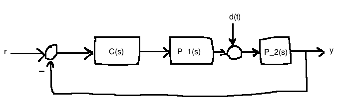
\[\begin{align} Y &= P_2(D+P_1C(-Y))\\ \frac{Y}{D} &= \frac{P_2}{1+P_1P_2C}\\ \end{align}\]
Suppose:
\[\begin{align}
D(s) &= \frac{N_d(s)}{D_d(s)}\\
&= \frac{N_d(s)}{D_d^-(s)D_d^+(s)}\\
\end{align}\]
Roots of \(D_d^+(s)\) have \(\Re(s) \ge 0\).
Assume IO stability so FVT applies:
\[\begin{align}
lim_{t\rightarrow\infty} y(t) &= \lim_{s \rightarrow 0}sY(s)\\
&= \lim_{s \rightarrow 0}s\frac{P_2(s)}{1+P_1P_2C}\frac{N_d}{D_d^-D_d^+}\\
&= \lim_{s \rightarrow 0}s\frac{N_{p_2}D_{p_1}D_c}{D_{p_2}D_{p_1}D_c+N_{p_1}N_{p_2}N_c}\frac{N_d}{D_d^-D_d^+}\\
\\
\mathcal{L}\{y\} &= Y(s)\\
\end{align}\]
So we see that to deal simultaneously with input and output disturbances, the controller must contain an internal model of \(D_d^+(s)\) (can't rely on the plant.) i.e.,
\[C(s)=\frac{1}{D_d^+(s)}C_1(s)\]
\[d(t)=1(t), \quad D(s)=\frac{1}{s}, \quad D_d^+(s)=s, \quad C(s)=\frac{1}{s}C_1(s)\]
\[D(t)=\sin(\omega t), \quad D(s)=\frac{\omega}{s^2+\omega^2}, \quad D_d^+(s)=s^2+\omega^2, \quad C(s)=\frac{1}{S^2+\omega^2}C_1(s)\]
\[D(t)=e^{-t}, \quad D(s)=\frac{1}{s+1}, \quad D_d^+(s)=1\]